Merging Spatial Data Sets

Like regular pandas DataFrames, GeoDataFrames can be merged with one another based on common merging variables. Unlike regular DataFrames, however, GeoDataFrames can also be merged based on spatial relationships using spatial joins with sjoin and sjoin_nearest.

Regular Merges

Regular merges (on attributes) work with dataframes in the familiar way, except that the syntax is just a little different. In particular, to merge a GeoDataFrame gdf with a DataFrame df, you would type gdf.merge(df, on="key") instead of the familiar pd.merge(gdf, df). This helps ensure that geopandas knows that you want to keep gdf as a geodataframe.

Spatial Join

The idea of a spatial join is that instead of joining rows across datasets based on common values of a variable, rows are joined based on spatial proximity. To illustrate, let’s being with two datasets: the dataset of countries we’ve been playing with already, and a dataset of cities:

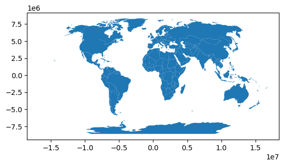
import geopandas as gpd

world = gpd.read_file(
    "https://github.com/nickeubank/practicaldatascience_book/"
    "raw/refs/heads/main/notebooks/"
    "gis/example_data/world_countries/world_countries_robinson.geojson"
)

world.plot()

<Axes: >

world.sample(3)

	featurecla	scalerank	labelrank	sovereignt	sov_a3	adm0_dif	level	type	tlc	admin	...	fclass_tr	fclass_id	fclass_pl	fclass_gr	fclass_it	fclass_nl	fclass_se	fclass_bd	fclass_ua	geometry
159	Admin-0 country	1	4	Antarctica	ATA	0	2	Indeterminate	1	Antarctica	...	None	None	None	None	None	None	None	None	None	MULTIPOLYGON (((-2950733.383 -7955019.899, -29...
34	Admin-0 country	1	5	Costa Rica	CRI	0	2	Sovereign country	1	Costa Rica	...	None	None	None	None	None	None	None	None	None	POLYGON ((-7765577.595 1023116.582, -7802508.3...
5	Admin-0 country	1	3	Kazakhstan	KA1	1	1	Sovereignty	1	Kazakhstan	...	None	None	None	None	None	None	None	None	None	POLYGON ((7202132.129 5245560.427, 7171298.638...

3 rows × 169 columns

cities = gpd.read_file(
    "https://github.com/nickeubank/practicaldatascience_book/raw"
    "/refs/heads/main/notebooks/gis/example_data/world_cities/world_cities_robinson.geojson"
)

cities.plot()

<Axes: >

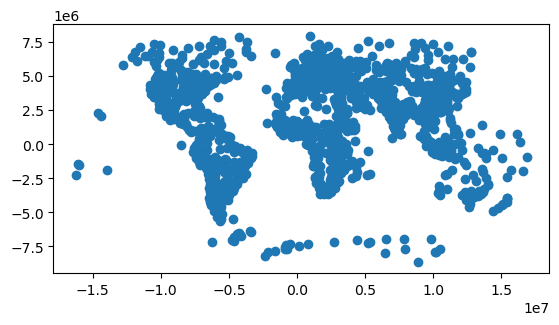
cities.sample(5)

	scalerank	natscale	labelrank	featurecla	name	namepar	namealt	nameascii	adm0cap	capin	...	fclass_id	fclass_pl	fclass_gr	fclass_it	fclass_nl	fclass_se	fclass_bd	fclass_ua	fclass_tlc	geometry
821	3	110	5	Admin-1 capital	Fez	None	Fes|F-s	Fez	0	None	...	None	None	None	None	None	None	None	None	None	POINT (-447202.186 3642475.12)
1194	1	300	7	Admin-1 capital	Geneva	None	None	Geneva	0	None	...	None	None	None	None	None	None	None	None	None	POINT (516080.209 4932107.829)
298	4	50	5	Admin-1 capital	Oujda	None	None	Oujda	0	None	...	None	None	None	None	None	None	None	None	None	POINT (-170321.402 3710190.811)
723	4	50	8	Populated place	Manukau	None	Southern Auckland	Manukau	0	None	...	None	None	None	None	None	None	None	None	None	POINT (15444681.861 -3956875.686)
494	4	50	1	Populated place	Hailar	None	None	Hailar	0	None	...	None	None	None	None	None	None	None	None	None	POINT (9869316.008 5244003.816)

5 rows × 138 columns

In this toy city dataset, you will notice that we have cities’ names, but not the country in which they are located. Since we know this variable is in our world dataset, we can do a spatial join to match each city observation up with the country in which it is located:

cities_w_county = cities.sjoin(world, how="left", predicate="intersects")
cities_w_county.sample(3)

	scalerank_left	natscale	labelrank_left	featurecla_left	name_left	namepar	namealt	nameascii	adm0cap	capin	...	fclass_vn_right	fclass_tr_right	fclass_id_right	fclass_pl_right	fclass_gr_right	fclass_it_right	fclass_nl_right	fclass_se_right	fclass_bd_right	fclass_ua_right
368	4	50	2	Populated place	Torreón	None	Torreon	Torreon	0	None	...	None	None	None	None	None	None	None	None	None	None
383	4	50	2	Admin-1 capital	Ibadan	None	None	Ibadan	0	None	...	None	None	None	None	None	None	None	None	None	None
794	3	110	8	Admin-0 capital	Dushanbe	None	None	Dushanbe	1	None	...	None	None	None	None	None	None	None	None	None	None

3 rows × 307 columns

Voilá! Just like that we’ve merged two datasets that have no variables in common.

Note that like our regular merge/join methods, we can use how to dictate which observations remain in our joined dataset. Unlike a regular merge/join, though, we also have the argument predicate which dictates what spatial relationships should be merged. When merging points with polygons, there aren’t a lot of ways you can imagine rows relating to one another. But spatial joins can also be done with lines and polygons (say, matching roads with the states they cross), or with polygons and polygons (matching media markets to states), and in those settings you can imagine more complicated relationships. For example, perhaps we only want to join roads to states if the road lies entirely within the state; or perhaps we want to join our roads to any state they touch. To accommodate these different relationships, predicate accepts:

• intersects

• contains

• within

• touches

• crosses

• overlaps

Order of Join

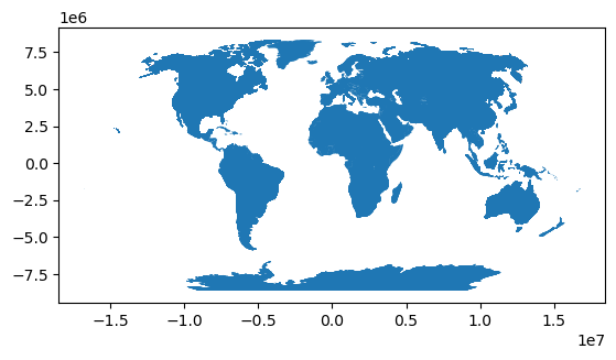
Note that while normal merge/join are symmetric – it doesn’t really matter which is the right dataset and which is left – order does matter for spatial joins, as only the geometry of one dataset is preserved. So if we do cities.sjoin(world), the resulting geodataframe will be points (as above). But if we flip the order, we end up with country polygons:

world.sjoin(cities).plot()

<Axes: >

Nearest Spatial Join

sjoin is terrific for linking observations that are in the same location. But sometimes we’re interested not in joining records that are in exactly the same spot or are overlapping, but rather observations that are near to one another.

For that, geopandas has sjoin_nearest. sjoin_nearest, as the name implies, merges an observation in one dataset to the nearest observation in another dataset.

To illustrate, let’s find out what city is closest to the “middle” of each country (e.g. closest to each country’s centroid):

world["centroids"] = world.centroid
world = world.set_geometry("centroids")
center_most_city = world.sjoin_nearest(cities, how="inner")
center_most_city = center_most_city.rename(columns={"name_right": "centermost_city"})
center_most_city.sample(3)

	featurecla_left	scalerank_left	labelrank_left	sovereignt	sov_a3_left	adm0_dif	level	type	tlc	admin	...	fclass_tr_right	fclass_id_right	fclass_pl_right	fclass_gr_right	fclass_it_right	fclass_nl_right	fclass_se_right	fclass_bd_right	fclass_ua_right	fclass_tlc_right
21	Admin-0 country	1	3	Norway	NOR	0	2	Sovereign country	None	Norway	...	None	None	None	None	None	None	None	None	None	None
77	Admin-0 country	1	5	Lebanon	LBN	0	2	Sovereign country	1	Lebanon	...	None	None	None	None	None	None	None	None	None	None
157	Admin-0 country	1	3	Yemen	YEM	0	2	Sovereign country	1	Yemen	...	None	None	None	None	None	None	None	None	None	None

3 rows × 308 columns

(Note we’re getting those same errors about calculating distances using a “geographic CRS” we got before. Once again, geopandas is telling us something important, and I definitely wouldn’t ignore these warnings in a real analysis. I just want to put off discussion of projections till a future reading.)

Voilá! Obviously this isn’t the most compelling illustrative example, but you could easily see how this might be helpful for, say, finding the supply depots closest to each store, the polling place closest to each voter, etc.

Geometric Manipulations

As we saw above, geopandas has utilities (like .centroid) for manipulating the geometric objects. The full like of supported manipulations can be found here, but some of the most useful are:

• generating centroids (.centroid),

• calculating geometric properties like area or length (.area and .length), and

• dissolving all the distinct geometries in a geodataframe into a single shape (.unary_union).

Perhaps the most useful for relating data, though, is .buffer(). Buffer takes a set of points and converts them into circular polygons of a given radius. This is extremely useful if you, say, want to do a spatial join to find all the observations in another dataset that are within a given distance of your original points.

To illustrate, suppose you wanted to find all the cities within 500 kilometers of each city in our cities dataset – how would you do it?

Well, we can start by using .buffer() to create a new GeoDataFrame with circular polygons instead of points. Then we can do a spatial join of that new GeoDataFrame with our original cities GeoDataFrame to find all the cities that intersect each city’s 500 km circle.

And now we can do our buffer and join:

# Create circular polygons with buffer
cities["buffers"] = cities.buffer(500_000)

# Make the buffers the "official geometry"
city_buffers = cities.set_geometry("buffers")
city_buffers.plot()

<Axes: >

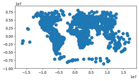
I know that plot looks very similar to the one above, but that’s just an illusion of the plots – the plot we created before buffering turned our points into circles to help visualize them, but from the perspective of geopandas, they’re just points with zero area. Now that we’ve buffered them, however, they’re actually polygons with diameters of 500 kilometers:

city_buffers.sample(3)

	scalerank	natscale	labelrank	featurecla	name	namepar	namealt	nameascii	adm0cap	capin	...	fclass_pl	fclass_gr	fclass_it	fclass_nl	fclass_se	fclass_bd	fclass_ua	fclass_tlc	geometry	buffers
1014	3	110	3	Admin-1 capital	Córdoba	None	None	Cordoba	0	None	...	None	None	None	None	None	None	None	None	POINT (-5794464.222 -3358121.98)	POLYGON ((-5294464.222 -3358121.98, -5296871.8...
808	3	110	7	Admin-1 capital	Trondheim	None	None	Trondheim	0	None	...	None	None	None	None	None	None	None	None	POINT (759993.731 6666421.27)	POLYGON ((1259993.731 6666421.27, 1257586.094 ...
364	4	50	2	Populated place	Okha	None	None	Okha	0	None	...	None	None	None	None	None	None	None	None	POINT (11409502.597 5693743.277)	POLYGON ((11909502.597 5693743.277, 11907094.9...

3 rows × 139 columns

With areas of \(500,000^2 \pi = 7.84 * 10^{11}\) meters squared:

city_buffers.sample(3).area

558    7.841371e+11
863    7.841371e+11
475    7.841371e+11
dtype: float64

So now we can do a spatial join of these circular polygons with our city points, and any cities that intersect with these buffers will be matched up, giving us a dataset of cities and their neighbors!

# Now join the polygons with our points
joined = cities.sjoin(city_buffers[["name", "buffers"]])
joined.sample(5)

	scalerank	natscale	labelrank	featurecla	name_left	namepar	namealt	nameascii	adm0cap	capin	...	fclass_it	fclass_nl	fclass_se	fclass_bd	fclass_ua	fclass_tlc	geometry	buffers	index_right	name_right
278	4	50	8	Admin-0 capital	Ljubljana	None	None	Ljubljana	1	None	...	None	None	None	None	None	None	POINT (1221166.524 4915887.993)	POLYGON ((1721166.524 4915887.993, 1718758.888...	1234	Rome
1119	2	200	1	Admin-1 capital	Bandung	None	None	Bandung	0	None	...	None	None	None	None	None	None	POINT (10137857.041 -743110.828)	POLYGON ((10637857.041 -743110.828, 10635449.4...	438	Malang
261	4	50	5	Admin-1 capital	Iquitos	None	None	Iquitos	0	None	...	None	None	None	None	None	None	POINT (-6914602.072 -401071.579)	POLYGON ((-6414602.072 -401071.579, -6417009.7...	968	Cruzeiro do Sul
533	4	50	3	Admin-1 region capital	Bordeaux	None	None	Bordeaux	0	None	...	None	None	None	None	None	None	POINT (-50589.332 4789505.008)	POLYGON ((449410.668 4789505.008, 447003.032 4...	38	Rouen
669	4	50	5	Admin-1 capital	Annaba	None	None	Annaba	0	None	...	None	None	None	None	None	None	POINT (685551.281 3948344.194)	POLYGON ((1185551.281 3948344.194, 1183143.645...	21	Cagliari

5 rows × 141 columns

# Cleanup columns
joined = joined.rename(
    {"name_left": "city_name", "name_right": "nearby_city"}, axis="columns"
)
joined = joined.drop(["index_right", "buffers"], axis="columns")

# Cities are obviously within 500 kilometers of themselves, so
# drop the "self joins"
joined = joined[~(joined.city_name == joined.nearby_city)]

# Now check out a few!
joined.sort_values("city_name")

	scalerank	natscale	labelrank	featurecla	city_name	namepar	namealt	nameascii	adm0cap	capin	...	fclass_pl	fclass_gr	fclass_it	fclass_nl	fclass_se	fclass_bd	fclass_ua	fclass_tlc	geometry	nearby_city
346	4	50	2	Admin-1 capital	Abakan	None	None	Abakan	0	None	...	None	None	None	None	None	None	None	None	POINT (7291145.466 5706949.325)	Novokuznetsk
346	4	50	2	Admin-1 capital	Abakan	None	None	Abakan	0	None	...	None	None	None	None	None	None	None	None	POINT (7291145.466 5706949.325)	Kyzyl
346	4	50	2	Admin-1 capital	Abakan	None	None	Abakan	0	None	...	None	None	None	None	None	None	None	None	POINT (7291145.466 5706949.325)	Krasnoyarsk
1165	2	200	8	Admin-0 capital	Abidjan	None	None	Abidjan	1	De facto, admin	...	None	None	None	None	None	None	None	None	POINT (-379224.555 569318.534)	Yamoussoukro
1165	2	200	8	Admin-0 capital	Abidjan	None	None	Abidjan	1	De facto, admin	...	None	None	None	None	None	None	None	None	POINT (-379224.555 569318.534)	Bouaké
...	...	...	...	...	...	...	...	...	...	...	...	...	...	...	...	...	...	...	...	...	...
1208	1	300	2	Admin-1 region capital	Ōsaka	None	Osaka-Kobe	Osaka	0	None	...	None	None	None	None	None	None	None	None	POINT (12083472.403 3710306.48)	Kyoto
1208	1	300	2	Admin-1 region capital	Ōsaka	None	Osaka-Kobe	Osaka	0	None	...	None	None	None	None	None	None	None	None	POINT (12083472.403 3710306.48)	Hiroshima
1208	1	300	2	Admin-1 region capital	Ōsaka	None	Osaka-Kobe	Osaka	0	None	...	None	None	None	None	None	None	None	None	POINT (12083472.403 3710306.48)	Matsuyama
1208	1	300	2	Admin-1 region capital	Ōsaka	None	Osaka-Kobe	Osaka	0	None	...	None	None	None	None	None	None	None	None	POINT (12083472.403 3710306.48)	Miyazaki
1208	1	300	2	Admin-1 region capital	Ōsaka	None	Osaka-Kobe	Osaka	0	None	...	None	None	None	None	None	None	None	None	POINT (12083472.403 3710306.48)	Fukuoka

9078 rows × 139 columns

And that’s how we can compose operations to do some pretty amazing things!