Merging Spatial Data Sets

Like regular pandas DataFrames, GeoDataFrames can be merged with one another based on common merging variables. Unlike regular DataFrames, however, GeoDataFrames can also be merged based on spatial relationships using spatial joins with sjoin and sjoin_nearest.

Regular Merges

Regular merges (on attributes) work with dataframes in the familiar way, except that the syntax is just a little different. In particular, to merge a GeoDataFrame gdf with a DataFrame df, you would type gdf.merge(df, on="key") instead of the familiar pd.merge(gdf, df). This helps ensure that geopandas knows that you want to keep gdf as a geodataframe.

Spatial Join

The idea of a spatial join is that instead of joining rows across datasets based on common values of a variable, rows are joined based on spatial proximity. To illustrate, let’s being with two datasets: the dataset of countries we’ve been playing with already, and a dataset of cities:

import geopandas as gpd
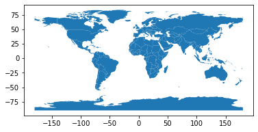
world = gpd.read_file(gpd.datasets.get_path('naturalearth_lowres'))
world.plot()

<AxesSubplot:>

world.sample(3)

	pop_est	continent	name	iso_a3	gdp_md_est	geometry
155	126451398	Asia	Japan	JPN	4932000.0	MULTIPOLYGON (((141.88460 39.18086, 140.95949 ...
30	11138234	South America	Bolivia	BOL	78350.0	POLYGON ((-69.52968 -10.95173, -68.78616 -11.0...
42	591919	South America	Suriname	SUR	8547.0	POLYGON ((-54.52475 2.31185, -55.09759 2.52375...

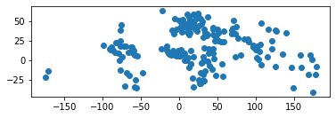
cities = gpd.read_file(gpd.datasets.get_path('naturalearth_cities'))
cities.plot()

<AxesSubplot:>

cities.sample(5)

	name	geometry
27	Bujumbura	POINT (29.36001 -3.37609)
23	Djibouti	POINT (43.14800 11.59501)
134	Ankara	POINT (32.86245 39.92918)
97	Vientiane	POINT (102.59998 17.96669)
73	Amman	POINT (35.93135 31.95197)

In this toy city dataset, you will notice that we have cities’ names, but not the country in which they are located. Since we know this variable is in our world dataset, we can do a spatial join to match each city observation up with the country in which it is located:

cities_w_county = cities.sjoin(world, how="left", predicate='intersects')
cities_w_county.sample(3)

	name_left	geometry	index_right	pop_est	continent	name_right	iso_a3	gdp_md_est
189	Cape Town	POINT (18.43304 -33.91807)	25.0	54841552.0	Africa	South Africa	ZAF	739100.0
200	Santiago	POINT (-70.66899 -33.44807)	10.0	17789267.0	South America	Chile	CHL	436100.0
50	Niamey	POINT (2.11471 13.51865)	55.0	19245344.0	Africa	Niger	NER	20150.0

Voilá! Just like that we’ve merged two datasets that have no variables in common.

Note that like our regular merge/join methods, we can use how to dictate which observations remain in our joined dataset. Unlike a regular merge/join, though, we also have the argument predicate which dictates what spatial relationships should be merged. When merging points with polygons, there aren’t a lot of ways you can imagine rows relating to one another. But spatial joins can also be done with lines and polygons (say, matching roads with the states they cross), or with polygons and polygons (matching media markets to states), and in those settings you can imagine more complicated relationships. For example, perhaps we only want to join roads to states if the road lies entirely within the state; or perhaps we want to join our roads to any state they touch. To accommodate these different relationships, predicate accepts:

• intersects

• contains

• within

• touches

• crosses

• overlaps

Order of Join

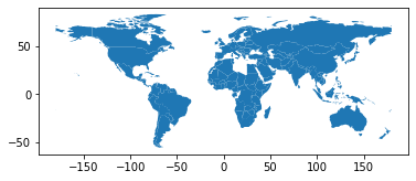
Note that while normal merge/join are symmetric – it doesn’t really matter which is the right dataset and which is left – order does matter for spatial joins, as only the geometry of one dataset is preserved. So if we do cities.sjoin(world), the resulting geodataframe will be points (as above). But if we flip the order, we end up with country polygons:

world.sjoin(cities).plot()

<AxesSubplot:>

Nearest Spatial Join

sjoin is terrific for linking observations that are in the same location. But sometimes we’re interested not in joining records that are in exactly the same spot or are overlapping, but rather observations that are near to one another.

For that, geopandas has sjoin_nearest. sjoin_nearest, as the name implies, merges an observation in one dataset to the nearest observation in another dataset.

To illustrate, let’s find out what city is closest to the “middle” of each country (e.g. closest to each country’s centroid):

world["centroids"] = world.centroid
world = world.set_geometry("centroids")
center_most_city = world.sjoin_nearest(cities, how="inner")
center_most_city = center_most_city.rename(
    {"name_right": "centermost_city"}, axis="columns"
)
center_most_city.sample(3)

/var/folders/tj/s8f2_ks15h315z5thvtnhz8r0000gp/T/ipykernel_40833/416860634.py:1: UserWarning: Geometry is in a geographic CRS. Results from 'centroid' are likely incorrect. Use 'GeoSeries.to_crs()' to re-project geometries to a projected CRS before this operation.

  world["centroids"] = world.centroid
/Users/Nick/opt/miniconda3/lib/python3.9/site-packages/geopandas/array.py:341: UserWarning: Geometry is in a geographic CRS. Results from 'sjoin_nearest' are likely incorrect. Use 'GeoSeries.to_crs()' to re-project geometries to a projected CRS before this operation.

  warnings.warn(

	pop_est	continent	name_left	iso_a3	gdp_md_est	geometry	centroids	index_right	centermost_city
171	2103721	Europe	Macedonia	MKD	29520.0	POLYGON ((22.38053 42.32026, 22.88137 41.99930...	POINT (21.69790 41.60593)	25	Skopje
157	28036829	Asia	Yemen	YEM	73450.0	POLYGON ((52.00001 19.00000, 52.78218 17.34974...	POINT (47.53504 15.91323)	136	Sanaa
43	67106161	Europe	France	-99	2699000.0	MULTIPOLYGON (((-51.65780 4.15623, -52.24934 3...	POINT (-2.87670 42.46070)	166	Madrid

(Note we’re getting those same errors about calculating distances using a “geographic CRS” we got before. Once again, geopandas is telling us something important, and I definitely wouldn’t ignore these warnings in a real analysis. I just want to put off discussion of projections till a future reading.)

Voilá! Obviously this isn’t the most compelling illustrative example, but you could easily see how this might be helpful for, say, finding the supply depots closest to each store, the polling place closest to each voter, etc.

Geometric Manipulations

As we saw above, geopandas has utilities (like .centroid) for manipulating the geometric objects. The full like of supported manipulations can be found here, but some of the most useful are:

• generating centroids (.centroid),

• calculating geometric properties like area or length (.area and .length), and

• dissolving all the distinct geometries in a geodataframe into a single shape (.unary_union).

Perhaps the most useful for relating data, though, is .buffer(). Buffer takes a set of points and converts them into circular polygons of a given radius. This is extremely useful if you, say, want to do a spatial join to find all the observations in another dataset that are within a given distance of your original points.

To illustrate, suppose you wanted to find all the cities within 500 kilometers of each city in our cities dataset – how would you do it?

Well, we can start by using .buffer() to create a new GeoDataFrame with circular polygons instead of points. Then we can do a spatial join of that new GeoDataFrame with our original cities GeoDataFrame to find all the cities that intersect each city’s 500 km circle.

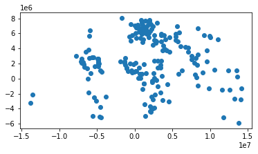
Note that to do this, I do have to play with the projection of our data a little. As we found before, our data is currently represented by x-y coordinates written in terms of degrees of latitude and longitude. But to create a buffer of 500 kilometers, we need to first move to a projection where the units are in meters, which I can do with .to_crs():

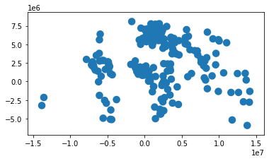
cities_reprojected = cities.to_crs("+proj=cea +lon_0=0 +lat_ts=45 +x_0=0 +y_0=0 +ellps=WGS84 +units=m +no_defs")
cities_reprojected.plot()

<AxesSubplot:>

And now we can do our buffer and join:

# Create circular polygons with buffer
cities_reprojected["buffers"] = cities_reprojected.buffer(500_000)

# Make the buffers the "official geometry"
city_buffers = cities_reprojected.set_geometry("buffers")
city_buffers.plot()

<AxesSubplot:>

I know that plot looks very similar to the one above, but that’s just an illusion of the plots – the plot we created before buffering turned our points into circles to help visualize them, but from the perspective of geopandas, they’re just points with zero area. Now that we’ve buffered them, however, they’re actually polygons with diameters of 500 kilometers:

city_buffers.sample(3)

	name	geometry	buffers
113	Cotonou	POINT (198539.858 997409.897)	POLYGON ((698539.858 997409.897, 696132.222 94...
39	Ashgabat	POINT (4603338.357 5510032.486)	POLYGON ((5103338.357 5510032.486, 5100930.721...
60	Honiara	POINT (12611532.802 -1466922.188)	POLYGON ((13111532.802 -1466922.188, 13109125....

With areas of \(500,000^2 \pi = 7.85 * 10^{11}\) meters squared:

city_buffers.sample(3).area

149    7.841371e+11
52     7.841371e+11
167    7.841371e+11
dtype: float64

So now we can do a spatial join of these circular polygons with our city points, and any cities that intersect with these buffers will be matched up, giving us a dataset of cities and their neighbors!

# Now join the polygons with our points
joined = cities_reprojected.sjoin(city_buffers[["name", "buffers"]])
joined.sample(5)

	name_left	geometry	buffers	index_right	name_right
4	Palikir	POINT (12469624.946 1077231.960)	POLYGON ((12969624.946 1077231.960, 12967217.3...	4	Palikir
87	Tallinn	POINT (1949727.750 7727330.615)	POLYGON ((2449727.750 7727330.615, 2447320.113...	154	Helsinki
86	Zagreb	POINT (1261548.941 6427274.597)	POLYGON ((1761548.941 6427274.597, 1759141.304...	86	Zagreb
192	Rome	POINT (984111.993 5985209.844)	POLYGON ((1484111.993 5985209.844, 1481704.357...	16	Ljubljana
21	Pristina	POINT (1668870.870 6074546.314)	POLYGON ((2168870.870 6074546.314, 2166463.233...	137	Bucharest

# Cleanup columns
joined = joined.rename(
    {"name_left": "city_name", "name_right": "nearby_city"}, axis="columns"
)
joined = joined.drop(["index_right", "buffers"], axis="columns")

# Cities are obviously within 500 kilometers of themselves, so
# drop the "self joins"
joined = joined[~(joined.city_name == joined.nearby_city)]

# Now check out a few!
joined.sort_values("city_name")

	city_name	geometry	nearby_city
156	Abidjan	POINT (-318698.444 829665.928)	Accra
156	Abidjan	POINT (-318698.444 829665.928)	Yamoussoukro
156	Abidjan	POINT (-318698.444 829665.928)	Lome
38	Abu Dhabi	POINT (4286633.823 3707394.154)	Doha
38	Abu Dhabi	POINT (4286633.823 3707394.154)	Manama
...	...	...	...
86	Zagreb	POINT (1261548.941 6427274.597)	Sarajevo
86	Zagreb	POINT (1261548.941 6427274.597)	Podgorica
86	Zagreb	POINT (1261548.941 6427274.597)	Budapest
86	Zagreb	POINT (1261548.941 6427274.597)	Belgrade
86	Zagreb	POINT (1261548.941 6427274.597)	Prague

410 rows × 3 columns

And that’s how we can compose operations to do some pretty amazing things!